Final

Author

Taylor Cote

In this project I wanted to look at the finances that go into college or relate to someones ability to go to college by state. I used data from college tuition by state, percentage of financial aid given by state and each states minimum wage. Knowing which states have the highest tuition is important when thinking about best value states to go to college. You can then compare this to the percent of financial aid given. I also thought have data on the minimum wage would be a goof factor to look at because many students work while in college to pay for it. All of these factors could help determine if a more expensive college in a state with a high percentage of financial aid and a high minimum wage might be worth it. I also looked at the different types of institutions. This can also allow someone to understand the weight of all of their options when picking a school and state to complete their higher education.

I first needed to set up before I started create visualizations. I loaded the packages I needed, data sets, set up a shape-file, changed column names and data to make sure everything matched and dropped na’s for all of the data sets.

library(tigris)
To enable caching of data, set `options(tigris_use_cache = TRUE)`
in your R script or .Rprofile.
library(leaflet)
library(tidyverse)
── Attaching core tidyverse packages ──────────────────────── tidyverse 2.0.0 ──
✔ dplyr     1.1.4     ✔ readr     2.1.5
✔ forcats   1.0.0     ✔ stringr   1.5.1
✔ ggplot2   3.5.1     ✔ tibble    3.2.1
✔ lubridate 1.9.3     ✔ tidyr     1.3.1
✔ purrr     1.0.2     
── Conflicts ────────────────────────────────────────── tidyverse_conflicts() ──
✖ dplyr::filter() masks stats::filter()
✖ dplyr::lag()    masks stats::lag()
ℹ Use the conflicted package (<http://conflicted.r-lib.org/>) to force all conflicts to become errors
library(sf)
Linking to GEOS 3.11.0, GDAL 3.5.3, PROJ 9.1.0; sf_use_s2() is TRUE
library(lubridate)
library(ggplot2)

college_cost <- read_csv('CollegeCost.csv')
Rows: 50 Columns: 12
── Column specification ────────────────────────────────────────────────────────
Delimiter: ","
chr  (1): states
num (11): 4pub-Total, 4pub-Tuition, 4pub-Room, 4pub-Board, 4priv-outstate, 4...

ℹ Use `spec()` to retrieve the full column specification for this data.
ℹ Specify the column types or set `show_col_types = FALSE` to quiet this message.
min_wage <- read_csv('MinWage.csv')
Rows: 50 Columns: 2
── Column specification ────────────────────────────────────────────────────────
Delimiter: ","
chr (1): State
dbl (1): State.Minimum.Wage.2020.Dollars

ℹ Use `spec()` to retrieve the full column specification for this data.
ℹ Specify the column types or set `show_col_types = FALSE` to quiet this message.
fin_aid <- read_csv('PercentFinAid.csv')
Rows: 51 Columns: 10
── Column specification ────────────────────────────────────────────────────────
Delimiter: ","
chr (10): State, Public, 4-year or above, Private not-for-profit, 4-year or ...

ℹ Use `spec()` to retrieve the full column specification for this data.
ℹ Specify the column types or set `show_col_types = FALSE` to quiet this message.
us_states <- states(cb = TRUE, resolution = "20m")
Retrieving data for the year 2021

  |                                                                            
  |                                                                      |   0%
  |                                                                            
  |=                                                                     |   1%
  |                                                                            
  |=======                                                               |   9%
  |                                                                            
  |=============                                                         |  18%
  |                                                                            
  |===================                                                   |  27%
  |                                                                            
  |=========================                                             |  36%
  |                                                                            
  |===============================                                       |  44%
  |                                                                            
  |=====================================                                 |  53%
  |                                                                            
  |===========================================                           |  62%
  |                                                                            
  |=================================================                     |  71%
  |                                                                            
  |========================================================              |  79%
  |                                                                            
  |==============================================================        |  88%
  |                                                                            
  |====================================================================  |  97%
  |                                                                            
  |======================================================================| 100%
college_cost |> 
  drop_na() -> college_cost

min_wage |> 
  drop_na() -> min_wage

fin_aid |> 
  drop_na() -> fin_aid

names(college_cost)
 [1] "states"                "4pub-Total"            "4pub-Tuition"         
 [4] "4pub-Room"             "4pub-Board"            "4priv-outstate"       
 [7] "4priv-Total"           "4priv-Tuition"         "4priv-Room"           
[10] "4priv-Board"           "2pub-instate-tuition"  "2pub-outstate-tuition"
names(college_cost)[which(names(college_cost) == "...1")] <- "State"

#college_cost <- college_cost %>%
#  mutate(states = tolower(states))

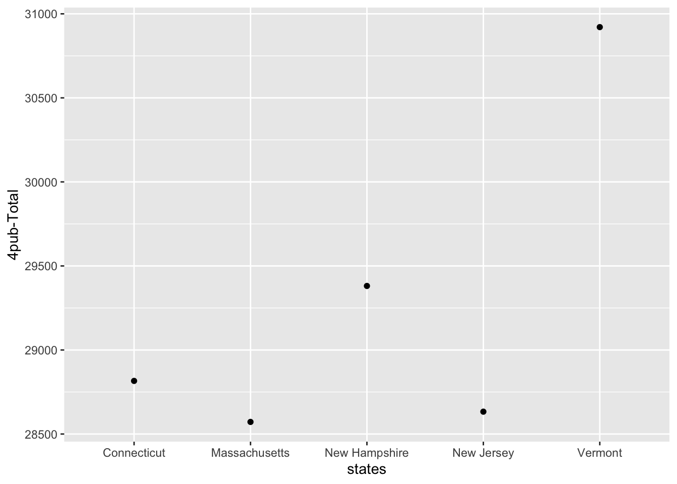
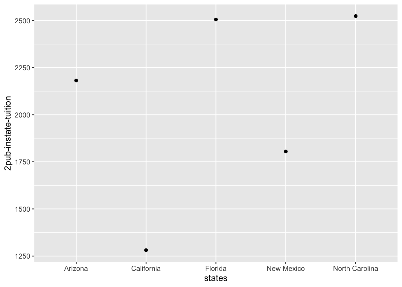
I then moved to working on visualizations. I started by merging the data. Finding the top 5 most and least expensive states for college tuition for a 4-year public school.

names(college_cost)[which(names(college_cost) == "...1")] <- "State"

cost <- merge(us_states, college_cost, by.x = "NAME", by.y = "states")

library(rmapshaper)

# reduce the number of points in your geometry
ms_simplify(cost) -> cost

top_5_costpub <- college_cost %>%
  arrange(desc(`4pub-Total`)) %>%
  head(5)

top_5_costpub %>% 
  ggplot(aes(states, `4pub-Total`)) + geom_point()

bottom_5_costpub <- college_cost %>%
  arrange(`4pub-Total`) %>%
  slice(1:5)

bottom_5_costpub %>% 
  ggplot(aes(states, `4pub-Total`)) + geom_point()

Vermont has the lowest cost of college for 4-year public institutions. While South Dakota has the highest cost.

I then wanted to see how every states college price compared on a map.

pal <- colorBin("Reds", domain = cost$`4pub-Total`, 6, pretty=TRUE)

cost |> 
st_transform('+proj=longlat +datum=WGS84') -> cost

leaflet(cost) %>%
  addTiles() %>%
  setView(-98.5795, 39.8282, zoom = 4) %>%  # center of U.S.A.
  addPolygons(
    fillColor = ~pal(cost$`4pub-Total`),
    fillOpacity = 0.7,
    stroke = TRUE,
    weight = 1,
    color = "black",
    label = ~paste0(NAME, ": $", `4pub-Total`),
    highlightOptions = highlightOptions(
      weight = 2,
      bringToFront = TRUE
    )
  )

I then did the same thing for each institution type.

4-Year Private

top_5_costpriv <- college_cost %>%
  arrange(desc(`4priv-Total`)) %>%
  head(5)

top_5_costpriv %>% 
  ggplot(aes(states, `4priv-Total`)) + geom_point()

bottom_5_costpriv <- college_cost %>%
  arrange(`4priv-Total`) %>%
  slice(1:5)

bottom_5_costpriv %>% 
  ggplot(aes(states, `4priv-Total`)) + geom_point()

Massachusetts has the highest cost for 4-year private institutions. While Idaho has the lowest.

pal <- colorBin("Reds", domain = cost$`4priv-Total`, 6, pretty=TRUE)

leaflet(cost) %>%
  addTiles() %>%
  setView(-98.5795, 39.8282, zoom = 4) %>%  # center of U.S.A.
  addPolygons(
    fillColor = ~pal(cost$`4priv-Total`),
    fillOpacity = 0.7,
    stroke = TRUE,
    weight = 1,
    color = "black",
    label = ~paste0(NAME, ": $", `4priv-Total`),
    highlightOptions = highlightOptions(
      weight = 2,
      bringToFront = TRUE
    )
  )

2-Year Public Instate

top_5_cost <- college_cost %>%
  arrange(desc(`2pub-instate-tuition`)) %>%
  head(5)

top_5_cost %>% 
  ggplot(aes(states, `2pub-instate-tuition`)) + geom_point()

bottom_5_cost <- college_cost %>%
  arrange(`2pub-instate-tuition`) %>%
  slice(1:5)

bottom_5_cost %>% 
  ggplot(aes(states, `2pub-instate-tuition`)) + geom_point()

New Hampshire has the highest cost for 2-year instate institutions. While Nebraska has the lowest cost for 2-year schools.

pal <- colorBin("Reds", domain = cost$`2pub-instate-tuition`, 6, pretty=TRUE)

leaflet(cost) %>%
  addTiles() %>%
  setView(-98.5795, 39.8282, zoom = 4) %>%  # center of U.S.A.
  addPolygons(
    fillColor = ~pal(cost$`2pub-instate-tuition`),
    fillOpacity = 0.7,
    stroke = TRUE,
    weight = 1,
    color = "black",
    label = ~paste0(NAME, ": $", `2pub-instate-tuition`),
    highlightOptions = highlightOptions(
      weight = 2,
      bringToFront = TRUE
    )
  )

2-Year Public Out of State

top_5_cost <- college_cost %>%
  arrange(desc(`2pub-outstate-tuition`)) %>%
  head(5)

top_5_cost %>% 
  ggplot(aes(states, `2pub-outstate-tuition`)) + geom_point()

bottom_5_cost <- college_cost %>%
  arrange(`2pub-outstate-tuition`) %>%
  slice(1:5)

bottom_5_cost %>% 
  ggplot(aes(states, `2pub-outstate-tuition`)) + geom_point()

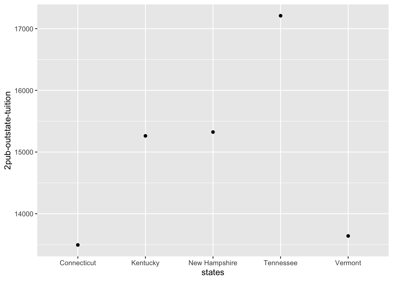
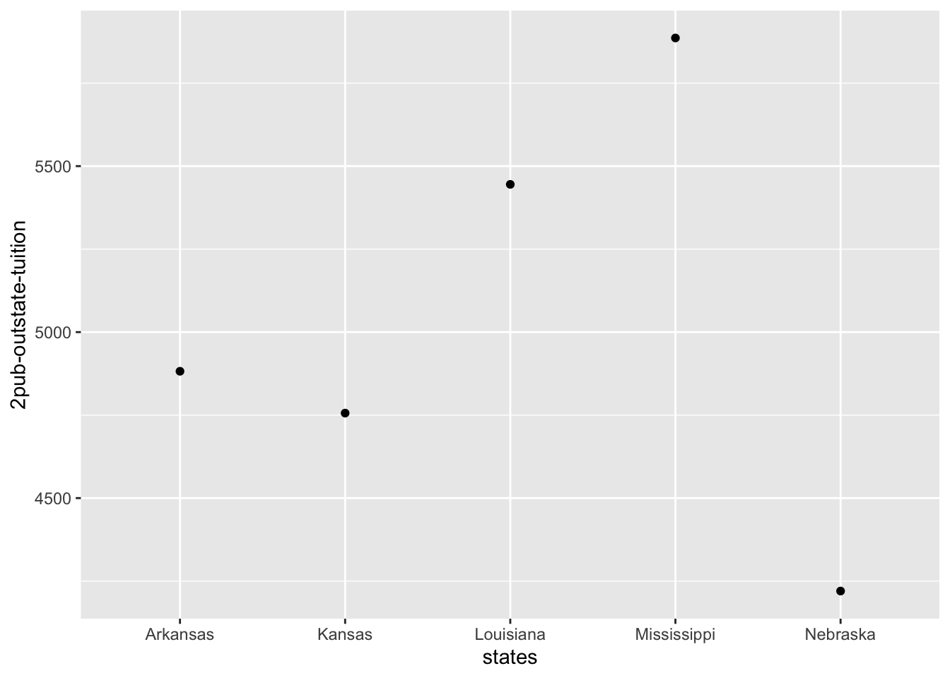
Tennessee has the highest cost for their 2-year out of state schools. While Mississippi has the lowest.

pal <- colorBin("Reds", domain = cost$`2pub-outstate-tuition`, 6, pretty=TRUE)

leaflet(cost) %>%
  addTiles() %>%
  setView(-98.5795, 39.8282, zoom = 4) %>%  # center of U.S.A.
  addPolygons(
    fillColor = ~pal(cost$`2pub-outstate-tuition`),
    fillOpacity = 0.7,
    stroke = TRUE,
    weight = 1,
    color = "black",
    label = ~paste0(NAME, ": $", `2pub-outstate-tuition`),
    highlightOptions = highlightOptions(
      weight = 2,
      bringToFront = TRUE
    )
  )

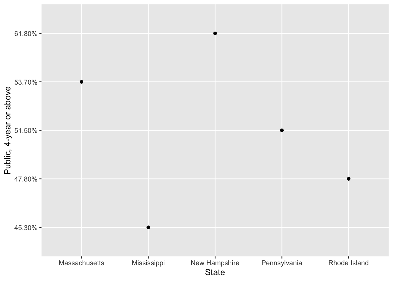
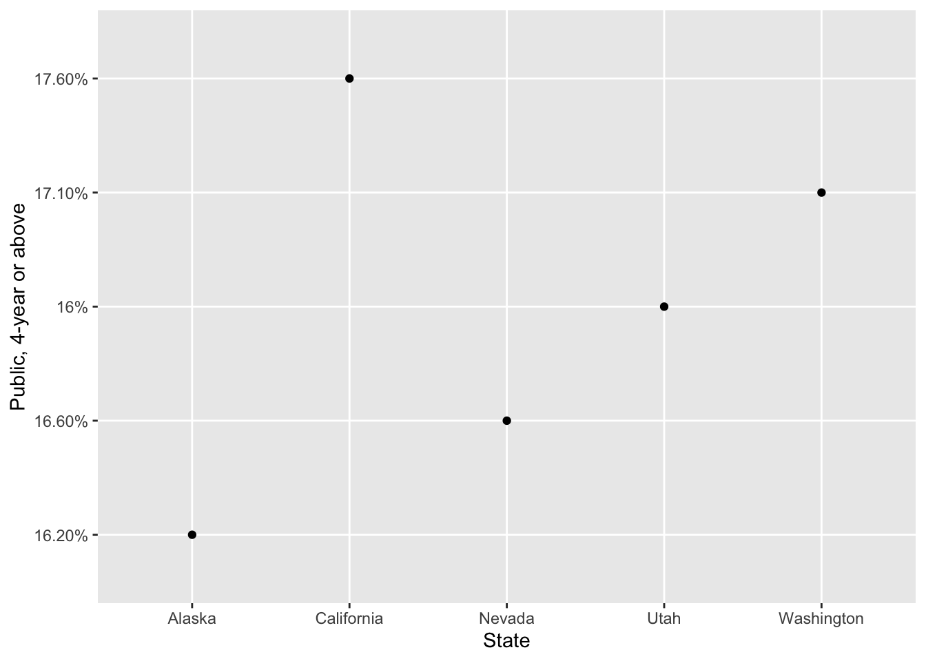
I then moved onto looking at the percent of financial aid given in each state. This needed to be mutated a bit because the percentage data did not graph so I converted that to be able to plot.

I did the same things. I looked at the top 5 states with the highest percent of financial aid, and the lowest 5. I also compared every state on a map.

#fin_aid <- fin_aid %>%
 # mutate(State = tolower(State))

finaid <- merge(us_states, fin_aid, by.x = "NAME", by.y = "State")

top_5_finaid <- fin_aid %>%
  arrange(desc(`Public, 4-year or above`)) %>%
  head(5)

top_5_finaid %>% 
  ggplot(aes(State, `Public, 4-year or above`)) + geom_point()

bottom_5_finaid <- fin_aid %>%
  arrange(`Public, 4-year or above`) %>%
  slice(1:5)

bottom_5_finaid %>% 
  ggplot(aes(State, `Public, 4-year or above`)) + geom_point()

New Hampshire has the highest percent of financial aid given, this matches the high cost of 2-year in state colleges and higher cost of the 4-year public colleges. While the lowest is Alaska, but they are not added on other maps.

finaid$`Public, 4-year or above` <- as.numeric(sub("%", "", finaid$`Public, 4-year or above`))


pal <- colorBin("Reds", domain = finaid$`Public, 4-year or above`, 6, pretty=TRUE)


# Check if conversion is successful
#str(finaid$`Public, 4-year or above`)


leaflet(finaid) %>%
  addTiles() %>%
  setView(-98.5795, 39.8282, zoom = 4) %>%  # center of U.S.A.
  addPolygons(
    fillColor = ~pal(`Public, 4-year or above`),
    fillOpacity = 0.7,
    stroke = TRUE,
    weight = 1,
    color = "black",
    label = ~paste0(NAME, ": %", `Public, 4-year or above`),
    highlightOptions = highlightOptions(
      weight = 2,
      bringToFront = TRUE
    )
  )
Warning: sf layer has inconsistent datum (+proj=longlat +datum=NAD83 +no_defs).
Need '+proj=longlat +datum=WGS84'

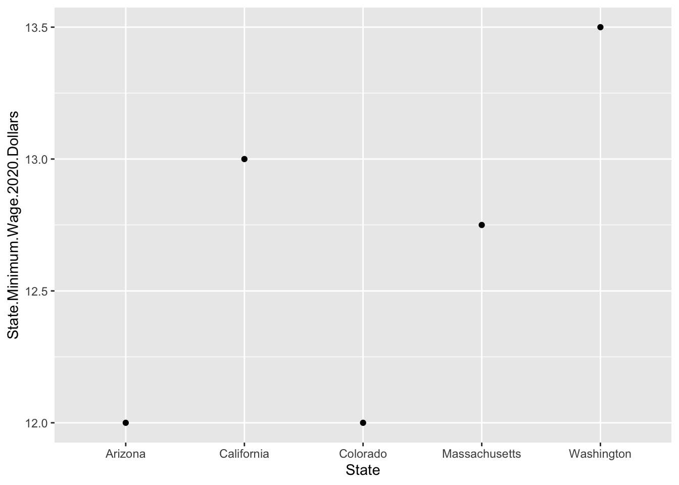
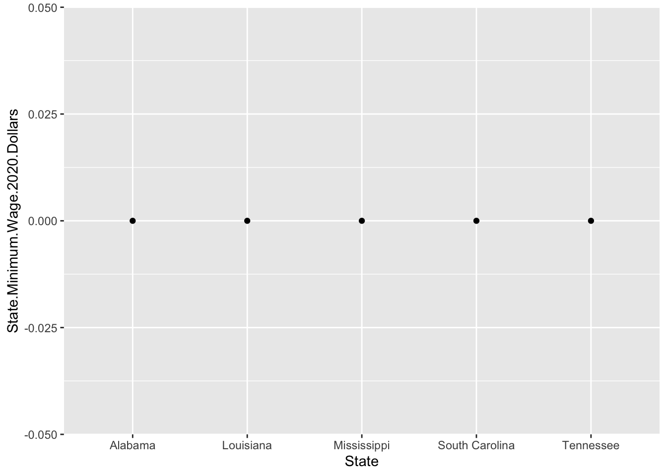
I then did the same to look at the top 5 highest and lowest minimum wage in each state and then a map of the minimum wage in each state.

#min_wage <- min_wage %>%
 # mutate(State = tolower(State))

wage <- merge(us_states, min_wage, by.x = "NAME", by.y = "State")

top_5_minwage <- min_wage %>%
  arrange(desc(`State.Minimum.Wage.2020.Dollars`)) %>%
  head(5)

top_5_minwage %>% 
  ggplot(aes(State, `State.Minimum.Wage.2020.Dollars`)) + geom_point()

bottom_5_minwage <- min_wage %>%
  arrange(`State.Minimum.Wage.2020.Dollars`) %>%
  slice(1:5)

bottom_5_minwage %>% 
  ggplot(aes(State, `State.Minimum.Wage.2020.Dollars`)) + geom_point()

Washington has the highest minimum wage. Massachusetts has the third highest which aligns with how high their 4-year private colleges are. There are 5 states that do not have a minimum wage and follow the national minimum wage. These are Alabama, Louisiana, Mississippi, South Carolina, and Tennessee. This aligns with the costs of institutions because none of these states are listed as having a high cost for schools.

pal <- colorBin("Reds", domain = wage$`State.Minimum.Wage.2020.Dollars`, 6, pretty=TRUE)

leaflet(wage) %>%
  addTiles() %>%
  setView(-98.5795, 39.8282, zoom = 4) %>%  # center of U.S.A.
  addPolygons(
    fillColor = ~pal(wage$`State.Minimum.Wage.2020.Dollars`),
    fillOpacity = 0.7,
    stroke = TRUE,
    weight = 1,
    color = "black",
    label = ~paste0(NAME, ": $", `State.Minimum.Wage.2020.Dollars`),
    highlightOptions = highlightOptions(
      weight = 2,
      bringToFront = TRUE
    )
  )
Warning: sf layer has inconsistent datum (+proj=longlat +datum=NAD83 +no_defs).
Need '+proj=longlat +datum=WGS84'

Overall, a lot of of the states with the higher percent of financial aid and minimum wage where also the ones with the higher costs for schools. This makes sense because a lot of college student rely on financial aid as well has a job to pay for school. I work in the same state that I attend school so for the minimum wage to be reasonable compared to the cost of school makes sense. It also helps when the percent of financial aid given aligns with the cost of the schools. I hope being able to see the costs of different institutions types, financial aid, and minimum wage for each state.